Home | Overview | Browser | Access | Login | Cookbook

Data Overview

The underlying content and schema of the archive are described below.

The VSA consists of a series of database releases. For information on these releases, content and sky coverge see the surveys page. More detailed information can be found in the papers accompanying the releases, see publications.

Users of the VSA data should note the limitations and known issues detailed under the release history.

Summary:
The pixel/image data are held in pipeline processed multi-extension FITS files (multiframes). Compressed library jpegs images are also generated and stored. VSA catalogue data are housed in a relational database running on Microsoft SQL Server 2008. Data are stored in tables which are inter-linked via reference ID numbers. In addition to the main astronomical object catalogues these tables also contain the meta-data of the multiframe images and calibration information.

The following sections discuss the structure and content of the VSA database. Further details can be found using the schema browser.

Jump to:

• Detailed overview
• frameTypes
• Tables
• Creating the merged tables (source merging and seaming)
• Quality error bit flags
• Magnitudes

VSA - Detailed Overview

Users wishing to work with the flat-files directly (i.e. the FITS images and catalogues) might find the flat file page helpful.

Multiframes will exist for all observation types e.g. darks, flats, science etc and data products e.g. stacks, mosaics, difference images etc. It should be noted that the FITS image extensions are mainly held as RICE compressed binary table extensions and that not all multiframes will have 16 four image extension e.g. mosaics/tiles.

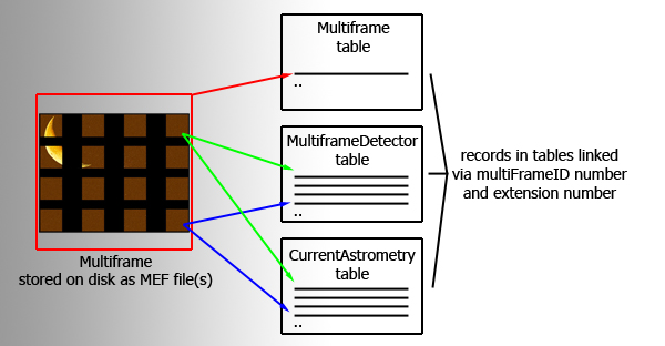
Schematic diagram of a multiframe

Multiframes are described in the database by entries in three main tables. The multiframe table primarily holds the meta-data that are applicable to a multiframe as a whole rather than an individual detector e.g. basic observation details. These meta-data originate from the primary header of the MEF file. Every multiframe held in archive is represented by a single row in the multiframe table with the attributes/columns in the row holding the meta-data. The multiframeDetector table contains details applicable to individual detector frames that are part of a multiframe. The third main table, currentAstrometry, contains the current astrometric calibration coefficients (WCS) for each science detector frame that is again part of a multiframe. If a multiframe has 16 detectors/extensions there will be 16 corresponding entries (rows) in multiframeDetector and currentAstrometry. A schematic representation of a multiframe is shown above

Each multiframe is assigned a unique ID number multiframeID which is an attribute in many tables held in the archive including each of the three tables discussed above (multiframe, multiframeDetector and currentAstrometry). The multiframeID number is used, often in conjunction with the extension number attribute (extNum) to link the multiframe records held across the tables.

An example: A stacked J-band VIRCAM science observation at a single pointing is generated by the pipeline which produces a MEF file that holds the image data and a MEF file holding the catalogue data. This observation constitutes a multiframe and is assigned a multiframeID, say 12345, at ingest into the archive. A single row entry is written into the multiframe table, attributes in the row include the multiframeID, the filename of the image MEF file, the filename of the catalogue MEF file, the number of detectors/extensions (in this case 16) and observational meta-data. For every detector/extension in the multiframe, rows are written into multiframeDetector and currentAstrometry tables. Each of the 16 rows written into these two tables contains the same multiframeID (12345) and the relevant extension number (numbered 2-17). So if we want to find the WCS coefficients for the 10th detector in this multiframe we would need to query the currentAstrometry table looking for a row that has multiframeID=12345 and extNum=11.

Frametypes

• normal - the basic 16 detectors/extensions pawprint observation
• stack - formed by co-averaging (stacking) a jitter sequence of nomals (a pawprint with 16 extensions)
• tilestack - formed by mosaicing (tiling) a sequence of 6 stacks to fill the pawprint gaps and generate a single extension image with increased depth in the overlap regions.
• deepstack formed by co-averaging (stacking) stacks on the same pointing to achieve increased depth (a pawprint with 16 extensions).
• tiledeepstack formed by mosaicing (tiling) a sequence of 6 deepstacks to fill the gaps and generate a single extension deep image.

The VIDEO consortium generates their own deep products which are ingested into the VSA and these are assigned frameType mosaicdeepstack (mosaicdeepstackconf)

Quality control - quality control is carried out prior to data releases. During that process data might be assigned a deprecation flag at the multiframe or multiframeDetector level. List of deprecation codes and their meaning

Catalogue data
Objects produced when source extraction is performed on a multiframe are ingested, one object per row, into the relevant survey detection table (see tables below). The detection table also holds the catalogues generated from deep stacks of repeated observations. All the survey detection tables contain similar attributes/columns with each row representing an object detected in one waveband at one epoch. Source merging (see Creating the merged tables) is carried out on the detection tables to produce the corresponding survey source table. A log of the source merging for a given survey is recorded in a further table. The source table holds an object's multi-waveband, multi-epoch parameters in one row. The source tables for different surveys contain different attributes as each survey requires a particular set of observations. For example the VHS survey requires observations in Y, J, H, Ks. To help reduce the width of the source tables the attributes held for an object in a given waveband/epoch is a subset of those recorded in the detection table. To recover the full set of parameters multiframeID, frameSetID and SeqNum numbers are provided to allow cross-referencing.

Note that for any deep or synoptic survey/projects (e.g. VIDEO, VVV, VMC) the source table is generated from the catalogues/detections derived from the tiledeepstacks.

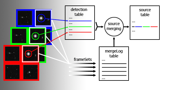
Schematic diagram of source merging via a frameSet

Taking the VHS as an example, the detections are held in vhsDetection, the source merging is recorded in vhsMergeLog and the merged sources placed in vhsSource. Imagine that three multiframes, taken in J, H, and Ks and covering approximately the same part of the sky, are produced by the pipeline. The multiframeIDs are say 12345, 23456 and 34567 respectively. Objects detected on each multiframe are loaded into vhsDetection. The multiframes are run through source merging which produces an entry in vhsMergeLog for each set of paired multiframe extensions. Typically the first extension in J will be paired with the first extensions of H and K. So looking at the pairing of the first extensions vhsMergeLog will contain an entry with a unique frameSetID, say 98765, which has attributes jmfID=12345, jeNum=2, hmfID=23456, heNum=2, kmfID=34567 and keNum=2. The records written into vhsSource by this pairing will all have frameSetID=98765. If we wanted to examine the full H band detection attributes of a given source in vhsSource that had say an hSeqNum=87654 we would first need know the extNum (e.g. 2) and H multiframeID (e.g. 23456), available by querying vhsMergeLog for frameSetID=98765 and then query vhsDetection for the entry corresponding to multiframeID=23456 extNum=2 and seqNum=87654.

The above description attempts to give users an overview of the tables they are most likely to use. The schema browser should be used to further explore the contents and layout of the archive.

VSA - Tables

Survey	Detection table	Source table	SynopticSource table	Variability table
VHS	vhsDetection	vhsSource	N/A	N/A
VMC	vmcDetection	vmcSource	vmcSynopticSource	vmcVariability
VVV	vvvDetection	vvvSource	vvvSynopticSource	vvvVariability
VIKING	vikingDetection	vikingSource	N/A	vikingVariability
VIDEO	videoDetection	videoSource	N/A	videoVariability

Source tables contain merged records from the deepest observations in each pointing for a given object in the passbands that define the survey. SynopticSource tables contain merged records from the contemporary colour observations in each pointing for a given object in the passbands that define the survey. Detection tables contain full details on the individual passband/epoch measurements. The source and detection tables are linked via reference multiframeID, extNum and seqNum values specifying the frame, extension and extraction order, e.g. a J-band observation in vvvSource has a jMfID, jeNum (both in vvvMergeLog, connected via frameSetID) and jSeqNum which are equal to multiframeID,extNum and seqNum in vvvDetection. The same is true for the SynopticSource tables. The Variability tables contain the statistics for multi-epoch observations, which allow selection on the variability properties. Variability tables are linked to Source tables via sourceID.

VSA - Source merging and seaming

Individual passband detections that come from VIRCAM images and that are stored in the *Detection tables in the VSA are automatically merged into multi-colour source lists stored in the *Source tables. The set of passbands is predefined for each survey and stored in the table RequiredFilters; that prescription is used to associate individual passbands/epochs into frame sets.

The core of the source merging algorithm uses a simple pairing procedure between pairs of frames before producing the final merged list. For a given frame set, frames are considered in pairs (say frames A and B) moving from short to long wavelengths, and early to late epochs where appropriate, and pairs are made by looking for the nearest detection in B for every detection in A out to a maximum pairing tolerance specified for each survey. The default pairing radius is usually 2.0 arcsec; for certain programmes - e.g. VMC and VVV, the pairing radius is 1.0 arcsec (prior to October 2014 the VMC pairing radius was 2 arcsec). The pairing criterion for each programme is stored in table PROGRAMME in attribute pairingCriterion; note that this is in units of degrees. To find out the pairing criteria in arcsec for the programmes that form part of a released database product, simply use the following SQL:
SELECT dfsIDString,description,pairingCriterion*3600.0 AS radius
FROMProgramme

The pairing is only considered as safe if the detection in B is the nearest to the detection in A, AND if the detection in A is the nearest to the detection in B: i.e. two sets of pointers of the nearest object in B to every object in A, and vice versa, are produced, and only consistent pair pointers are used to associate pairs of objects. If detection Y in B is the nearest as seen from the position of detection X in A, but detection Z in A is the nearest as seen from the position of Y in B, then the association is not made and detection X in A will not be paired to any in B.

Source merging then proceeds when all pair combinations of available passbands in the frame set have had consistent pointer sets produced. The merging procedure is simply to start with the shortest wavelength detection set as a master set, and merge in the pairs pointed to by each of the slave pointer sets; subsequently, the next shortest wavelength set is considered as the master, and all detections not already merged in previously are considered as slaves amongst the remaining passband sets. This process continues until only unmerged detections in the final passband set are left, and these are written into the merged source list. Hence, every detection amongst all the images in the frame set will have one, and only one, entry somewhere amongst the set of merged sources.

Note that the pairing radius is large compared to the typical astrometric errors (and may be too large for a given science application). This is in order that moving sources (e.g. high proper motion objects) and sources with unusually high centroiding errors (e.g. very faint and/or extended, low surface brightness objects) will be paired up in the merged source lists. The negative side to this is that some level of spurious matchings will inevitably occur. For well exposed, non-moving sources, some indication of the reliability of the merged set can be checked at usage (query) time by applying filters to the *Xi and *Eta attributes in the *Source table. These attributes provide the offset from master to slave for pairings, in arcsec, and should not be larger than about 1 arcsec for non-moving, well exposed sources. If your particular science application requires a more restrictive pairing tolerance, then simply tune by selecting on *Xi and *Eta at query time:
SELECT...WHERE jXi BETWEEN -1.0 AND +1.0 ...
etc.

Seaming - the final stage in the source table creation is to perform seaming which flags duplicate objects by populating the priOrSec (primary or secondary) flag. Matching objects in overlap regions are ranked according to their filter coverage then their quality error bit flags and finally their proximity to a detector edge. For example say the same source is found on three overlapping framesets having framesetID = X, Y and Z. Framesets Y and Z have coverage in J, H and Ks bands and X only has the J band. The quality error bit information (*ppErrBits) shows that more confidence can be placed in the source produced by frameset Y. The conclusion for this source is that the measurement taken from frameset Y is the primary and those taken from X and Z are secondary. The priOrSec flag for all three sources is set to framesetID Y. Sources that do not have duplicate measurements have priOrSEc=0. The SQL where clause to select only primary sources (i.e. purge duplicates) is
.... where (priOrsec=0 or priOrSec=framesetID)

VSA - Quality Error bit flagging

VSA - Magnitudes

Kron and Petrosian magnitudes are underestimated for large galaxies, because the aperture is limited to the largest aperture radius, aperRad13 = 12 arcsec. This is the approximately the same size as the background estimation mesh, so larger apertures risk producing large errors due to poor background subtraction. There are a small number of bright objects which do have larger Kron and Petrosian radii. Most of these are flagged as saturated, but a small number (a few tens) have no errors. Generally these are isolated large, bright galaxies. It should be noted that the value of kronRad is the first moment of the surface brightness profile and the value of petroRad is when the radius at which the surface brightness in an annulus is 0.2 times the mean surface brightness. The apertures in which the flux is calculated is twice this radius in both cases.

Which magnitude should I use?

The best magnitude to use very much depends on the objects that are being studied and what type of analysis you are doing. E.g. are they point sources, are they extragalactic, do you want total fluxes, or the best colours?

The CASU photometry gives best results for point-sources which are not heavily blended. The VISTA photometric system is close to the Vega system, so extra-galactic astronomers should take care to transform to AB if necessary. The VegaToAB corrections can be found in the Filter table.

Point-sources

Stars

In high density regions PSF model magnitudes are preferable, but this has not been implimented in the standard CASU imcore extractor (and is unlikely ever to be), so the PSF (and Sersic) magnitude columns in the main Detection tables are default. However, the VMC (and in all likelihood the VVV) team are producing PSF magnitudes, which we store in separate tables, e.g. vmcPsfCatalogue. These go deeper in very crowded regions and give high signal-to-noise colours.

One correction not applied is the interstellar extinction, mainly because this is unknowable unless you have both a distance and a 3 dimensional extinction map. We have set up some infrastructure for 3-D interstellar extinction maps, and include a VVV generated map of the Galactic bulge. In the future more of these will be included. See PDF 3D Extinction Maps usage examples.

The standard colours in the Source table use the 1.0 arcsec aperture corrected (aperMag3) magnitudes: e.g. ymjPnt=(yAperMag3-jAperMag3) when both yAperMag3 and jAperMag3 are >0 and otherwise default.

QSOs

QSOs or very distant galaxies will also be point like, so the aperture corrected aperture magnitudes used for stars will also be appropriate. However, a total interstellar extinction correction, and perhaps a correction to AB magnitudes, is also necessary. The total extinction correction for each band is in the Source table. The extinction correction must be subtracted. K-corrections, which are used to correct magnitudes in a pass-band for objects at different redshifts to a common basis and internal extinction corrections are not included, and require more knowledge of the object type that we know in general.

e.g.